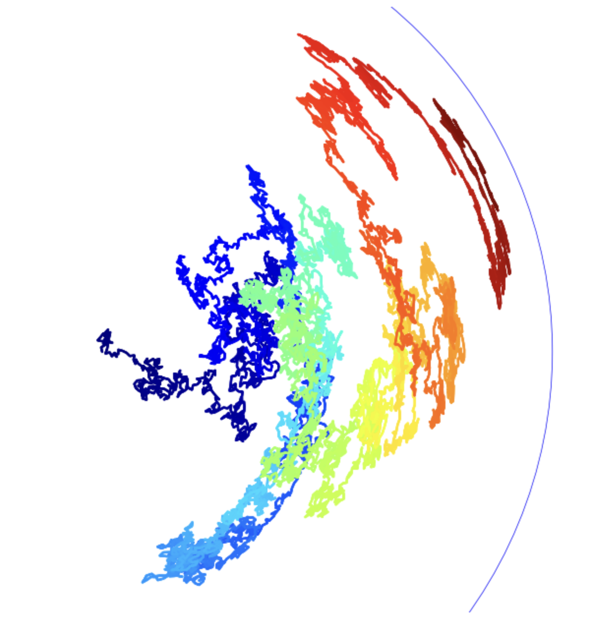
Random motion in the hyperbolic plane

The recipe

The standard brownian motion can be obtained by this recipe: look around you, choose at random a direction, make a tiny step in that direction and repeat from the beginning. When the stepsize goes to zero, you get the brownian motion. One can implement this in python, but it is worth trying something more involved, ie doing the same in the hyperbolic plane.

That space has a different geometry from the usual euclidean one. The hyperbolic plane has many descriptions and a common one is the disk model: the points of the space are all the points of the inside of the unit disk in the complex plane. When you are at a point $z$ in that unit disk, the way to measure distances is different: when the euclidean element of length was $|dz|$, it is now $\dfrac{|dz|}{1-|z|^2}$ in the hyperbolic plane. Observe that when $z=0$, the two ways of measuring distances actually coincide: we will use that later.

What are the consequences for a brownian path? Imagine that you travelled up to a point $a$. You want now to look around and choose a point randomly on the hyperbolic circle of small radius $\epsilon$, that is, the set of points lying at (hyperbolic) distance $\epsilon$ from $a$. It turns out that this set is still a circle, although not centered at $a$. But there is a trick you can use: move the point $a$ towards the origin by an isometry $M$ (a transformation that preserves the lengths and angles), observe that now that you are at the origin the set of equidistant points from the origin is a true standard circle centered at the origin, then pick your point at random on that circle, and move everything back by the inverse of the isometry you used.

The Möbius Transformation

The isometry sending $a$ towards the origin is called a Möbius transformation. It is defined as:

$M(z) = \frac{z-a}{1-\bar{a}z}$. Its inverse transformation is $M^{-1}(z) = \frac{z+a}{1+\bar{a}z}$.

The same in python:

def mobius(z, dz):
    return (z + dz) / (np.conjugate(dz) * z + 1)

The Core Function

To generate a path of points, we’ll create a function that iterates this transformation:

def mk_xy(epsilon=0.01, k=10, n=5000):
    z = complex(0.) #start at the origin
    path = [z]
    for t in range(n - 1):
        dz = epsilon * random_unit_vector()[0] # make a small step at random, from the origin
        z = mobius(z, dz) # send that small step back to the endpoint z of the path
        path.append(z)
    x, y = complex_path_to_real(path)
    # add extra points to improve the path's appearance
    x2, y2 = interpolate_path(x, y, n, k)
    # plot the path
    display_xy(x2, y2, n, k)

The result

The full script

import numpy as np
import matplotlib.pyplot as plt

DFLT_EPS = 0.01
DFLT_K = 10
DFLT_PTS = 5000

def mobius(z, dz):
    return (z + dz) / (np.conjugate(dz) * z +1)

def complex_path_to_real(path):
    return np.real(path), np.imag(path)

def random_unit_vector(size=1):
    theta = np.random.uniform(0., 1., size)
    return np.cos(2 * np.pi * theta) + 1j * np.sin(2 * np.pi * theta)

def mk_xy(epsilon=DFLT_EPS, k=DFLT_K, n=DFLT_PTS):
    z = 0j
    path = [z]
    for _ in range(n - 1):
        dz = epsilon * random_unit_vector()[0]
        z = mobius(z, dz)
        path.append(z)
    
    x, y = complex_path_to_real(np.array(path))
    x2, y2 = interpolate_path(x, y, n, k)
    display_xy(x2, y2, n, k)
    display_xy_save(x2, y2, n, k, filename="output.png")

def display_xy(x, y, n, k):
    fig, ax = plt.subplots(1, 1, figsize=(8, 8))
    ax.set_xlim((-1.1, 1.1))
    ax.set_ylim((-1.1, 1.1))
    circle = plt.Circle((0, 0), 1, color='b', fill=False, linewidth=0.5)
    ax.add_artist(circle)
    ax.scatter(x, y, c=range(n * k), linewidths=0, marker='o', s=3, cmap=plt.cm.jet)
    ax.axis('equal')
    ax.set_axis_off()
    ax.set_aspect(1)
    plt.show()
    

def interpolate_path(x, y, n, k):
    x2 = np.interp(np.arange(n * k), np.arange(n) * k, x)
    y2 = np.interp(np.arange(n * k), np.arange(n) * k, y)
    return x2, y2

def simple_run(n=DFLT_PTS):
    mk_xy(n=n)

# Example usage of the script
#simple_run(10000)